Few-Shot Learning And Zero-Shot Learning Equations Latex Code

Navigation

In this blog, we will summarize the latex code of most fundamental equations of Few-Shot Learning and Zero-Shot Learning. Few-Shot Learning learns from a few-labelled examples and better generalize to unseen examples. Typical works includes Prototypical Networks, Model-Agnostic Meta-Learning (MAML), etc.

• 1. Prototypical Networks (Protonets)
• 2. Model-Agnostic Meta-Learning (MAML)

• 1.1 Prototypes

  See paper Prototypical Networks for Few-shot Learning for more detail.

  Equation

  
  
  

  Latex Code

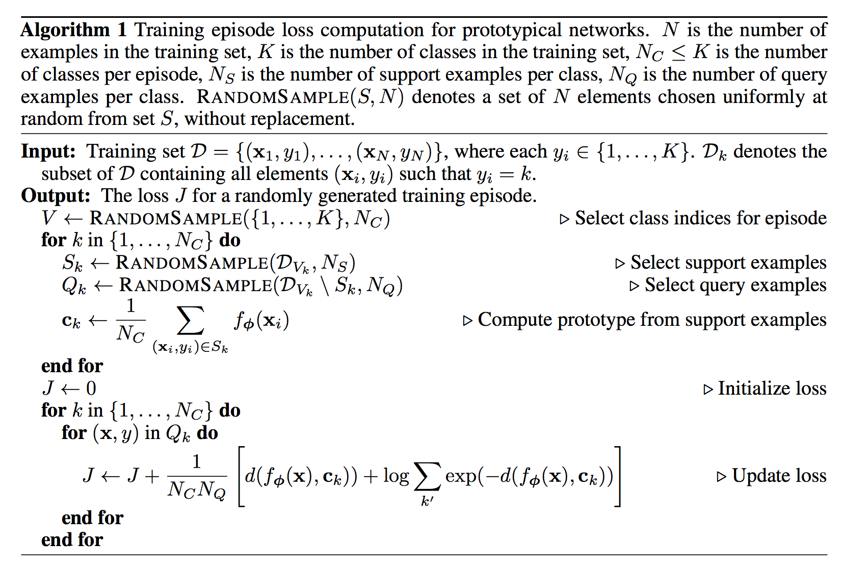
              c_{k}=\frac{1}{|S_{k}|}\sum_{(x_{i},y_{i}) \in S_{k}} f_{\phi}(x) \\ p_{\phi}(y=k|x)=\frac{\exp(-d(f_{\phi}(x), c_{k}))}{\sum_{k^{'}} \exp(-d(f_{\phi}(x), c_{k^{'}})} \\\min J(\phi)=-\log p_{\phi}(y=k|x)
          

  Explanation

  Prototypical networks compute an M-dimensional representation c_{k} or prototype, of each class through an embedding f_{\phi}(.) with parameters \phi. Each prototype is the mean vector of the embedded support points belonging to its class k. Prototypical networks then produce a distribution over classes for a query point x based on a softmax over distances to the prototypes in the embedding space as p(y=k|x). Then the negative log-likelihood of J(\theta) is calculated over query set.

  
  
  
  
  
  

  1.2 Prototypical Networks as Mixture Density Estimation

  Bregman divergences

  
  
  

              d_{\phi}(z,z^{'})=\phi(z) - \phi(z^{'})-(z-z^{'})^{T} \nabla \phi(z^{'})
          

  
  

  Mixture Density Estimation

  
  

              p_{\phi}(y=k|z)=\frac{\pi_{k} \exp(-d(z, \mu (\theta_{k})))}{\sum_{k^{'}} \pi_{k^{'}} \exp(-d(z, \mu (\theta_{k})))}
          

  Explanation

  The prototypi- cal networks algorithm is equivalent to performing mixture density estimation on the support set with an exponential family density. A regular Bregman divergence d_{\phi} is defined as above. \phi is a differentiable, strictly convex function of the Legendre type. Examples of Bregman divergences include squared Euclidean distance and Mahalanobis distance.

2. Model-Agnostic Meta-Learning (MAML)

• 1.1 MAML Meta-Objective

  Equation

  
  
  

  Latex Code

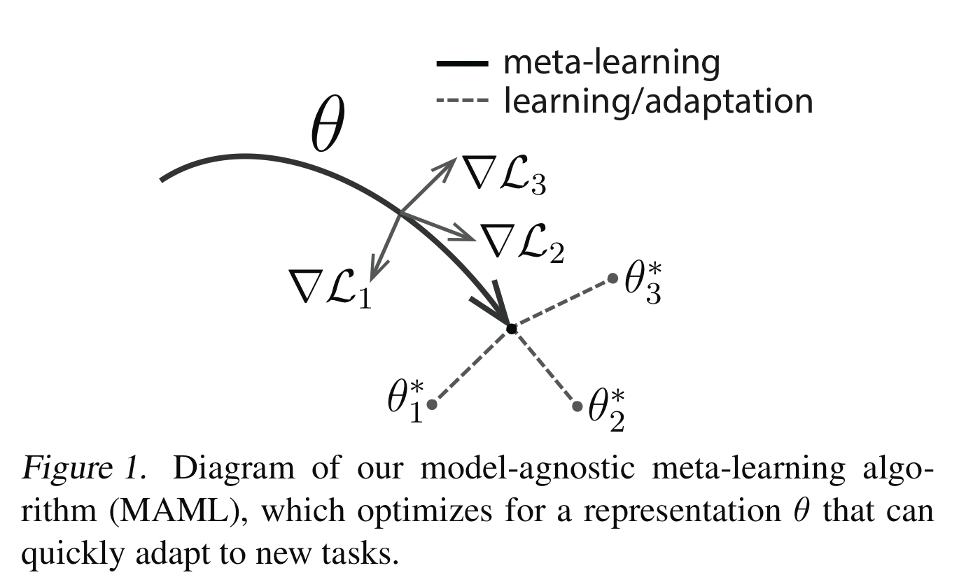
              \min_{\theta} \sum_{\mathcal{T}_{i} \sim p(\mathcal{T})} \mathcal{L}_{\mathcal{T}_{i}}(f_{\theta^{'}_{i}}) = \sum_{\mathcal{T}_{i} \sim p(\mathcal{T})} \mathcal{L}_{\mathcal{T}_{i}}(f_{\theta_{i} - \alpha \nabla_{\theta} \mathcal{L}_{\mathcal{T}_{i}} (f_{\theta}) })
          

  Explanation

  
  
  
  
  
  

  Model-Agnostic Meta-Learning (MAML) tries to find an initial parameter vector θ that can be quickly adapted via meta-task gradients to task-specific optimal parameter vectors. See paper Model-Agnostic Meta-Learning for Fast Adaptation of Deep Networks for details.